Fourier Transform
DFT: Discrete Fourier Transform
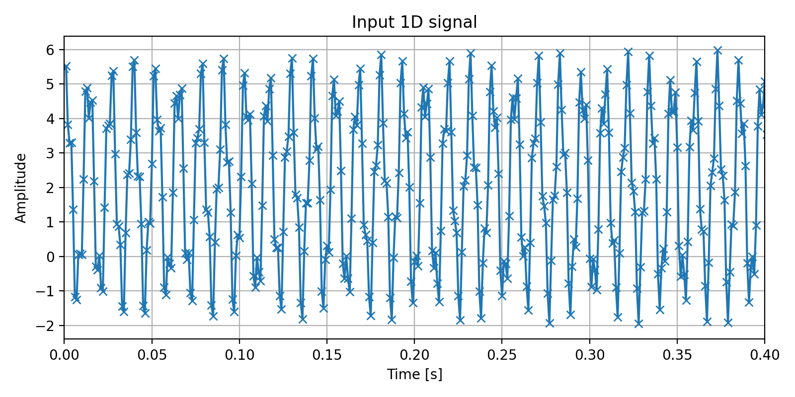
1D FFT Transform
import numpy as np
import matplotlib.pyplot as plt
# Sample Period/Frequency in second/hertz
Ts = 0.001
Fs = 1.0 / Ts
# Number of sample
N = 10000
# Time abscissa
t = np.arange(0, N) * Ts
# Example of a signal: sum of 2 sinus signal
# A1, A2: Amplitude (no unit)
# f1, f2: Frequency (Hertz)
# p1, p2: Phase (Radian)
# Offset
offset = 2.0
# 1st sinus parameters
A1 = 1.0
f1 = 255.0
p1 = 1.0
# 2nd sinus parameters
A2 = 3.0
f2 = 78.0
p2 = np.pi / 3.0
# Signal to analyse
x = offset
x += A1 * np.sin(2 * np.pi * f1 * t + p1)
x += A2 * np.sin(2 * np.pi * f2 * t + p2)
fig = plt.figure(figsize=(8, 4), tight_layout=True)
ax1 = fig.add_subplot(111)
ax1.set_title("Input signal")
ax1.set_xlabel("Time [s]")
ax1.set_ylabel("Amplitude")
ax1.grid()
ax1.plot(t, x, '-x')
ax1.set_xlim([0, 0.4])
fig.savefig("input_1d.png", dpi=200)
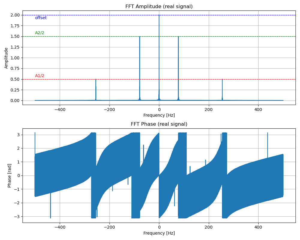
# Performing fast fourrier transform
fft_x = np.fft.fft(x, n=2**17)
# f = [-N/2, ..., -1, 0, 1, ..., N/2-1] / (Ts*N) if N is even
# f = [-(N-1)/2, ..., -1, 0, 1, ..., (N-1)/2] / (Ts*N) if N is odd
f = np.fft.fftshift(np.fft.fftfreq(len(fft_x), Ts))
abs_fft_x_unshifted = np.abs(fft_x)
angle_fft_x_unshifted = np.angle(fft_x)
abs_fft_x = np.fft.fftshift(abs_fft_x_unshifted)
angle_fft_x = np.fft.fftshift(angle_fft_x_unshifted)
# Fourier Series Coefficients Normalization
abs_fft_x_norm = abs_fft_x / N
fig = plt.figure(figsize=(10, 8))
fig.set_tight_layout('tight')
ax1 = fig.add_subplot(211)
ax1.set_xlabel("Frequency [Hz]")
ax1.set_ylabel("Amplitude")
ax1.set_title("FFT Amplitude (real signal)")
ax1.grid()
ax1.plot(f, abs_fft_x_norm)
ax1.axhline(offset, linewidth=1.0, linestyle='--', color='b',
label="offset amplitude")
ax1.axhline(A1 / 2.0, linewidth=1.0, linestyle='--', color='r',
label="sinusoide 1 amplitude")
ax1.axhline(A2 / 2.0, linewidth=1.0, linestyle='--', color='g',
label="sinusoide 2 amplitude")
ax1.text(f[0], offset - 0.1, "offset", color='b')
ax1.text(f[0], A1 / 2.0 + 0.05, "A1/2", color='r')
ax1.text(f[0], A2 / 2.0 + 0.05, "A2/2", color='g')
ax2 = fig.add_subplot(212, sharex=ax1)
ax2.set_xlabel("Frequency [Hz]")
ax2.set_ylabel("Phase [rad]")
ax2.set_title("FFT Phase (real signal)")
ax2.grid()
ax2.plot(f, angle_fft_x)
fig.savefig("fft_1d.png")
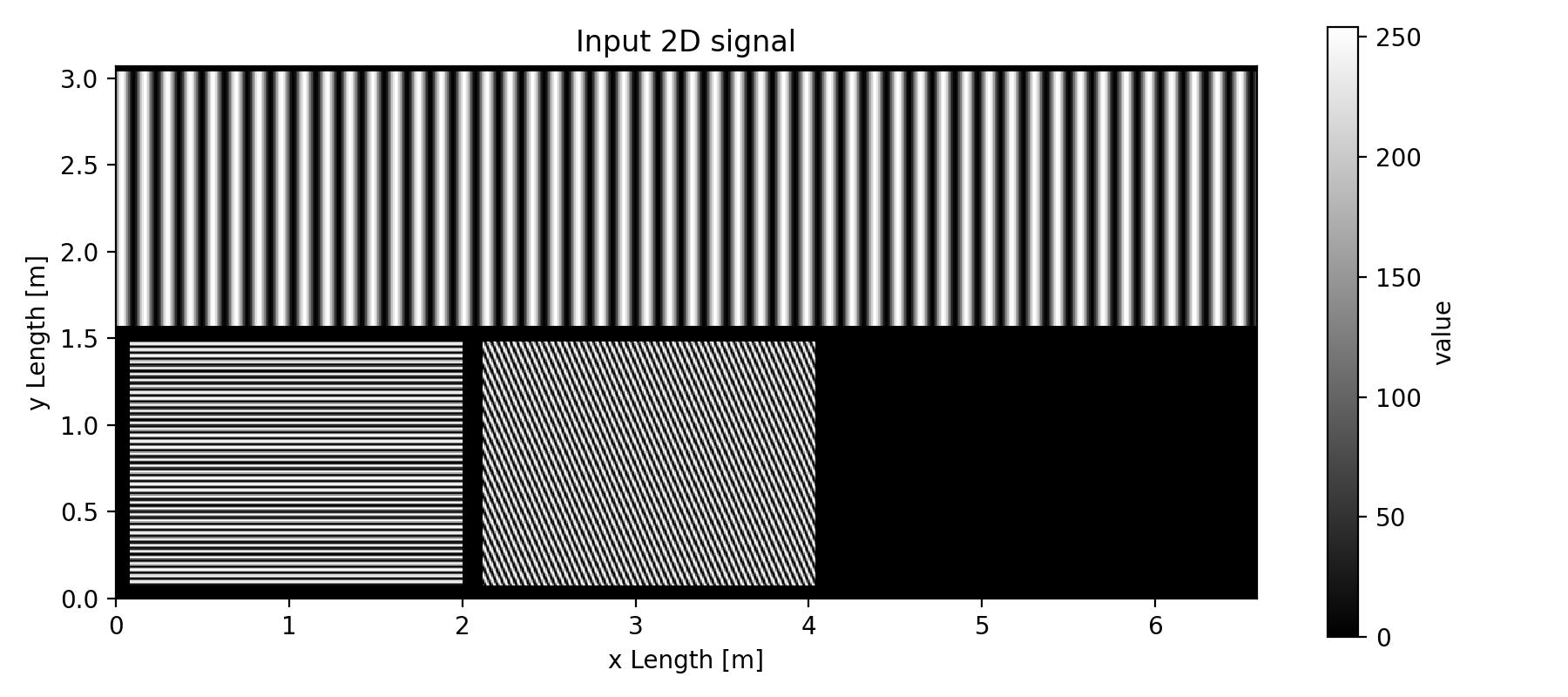
2D FFT Transform
Image used in this example:
Download: example.pgm.

import numpy as np
import matplotlib.pyplot as plt
from PIL import Image
plt.ioff()

# Loading the 2d data (the grayscale image in this case)
img_path = "example.png"
matrix_2d = np.array(Image.open(img_path))[::-1]

# Shape of the 2d data
N_y, N_x = matrix_2d.shape # N_y = 512 ; N_x = 823

# Sampling period [m] in both axis
# 8 mm
Ts_x = 8e-3
# 6 mm
Ts_y = 6e-3

# Plotting the 2d data (in this case the image)
fig = plt.figure(figsize=(9, 4), tight_layout=True)
ax1 = fig.add_subplot(111)
ax1.set_title("Input 2D signal")
ax1.set_xlabel("x Length [m]")
ax1.set_ylabel("y Length [m]")
# X and Y axis
x = np.arange(0, N_x + 1) * Ts_x
y = np.arange(0, N_y + 1) * Ts_y
pcolor = ax1.pcolormesh(x, y, matrix_2d, cmap="gray")
cbar = plt.colorbar(pcolor)
cbar.set_label('value')
ax1.set_aspect(1)
fig.savefig("input_2d.png", dpi=200)
plt.close(fig)
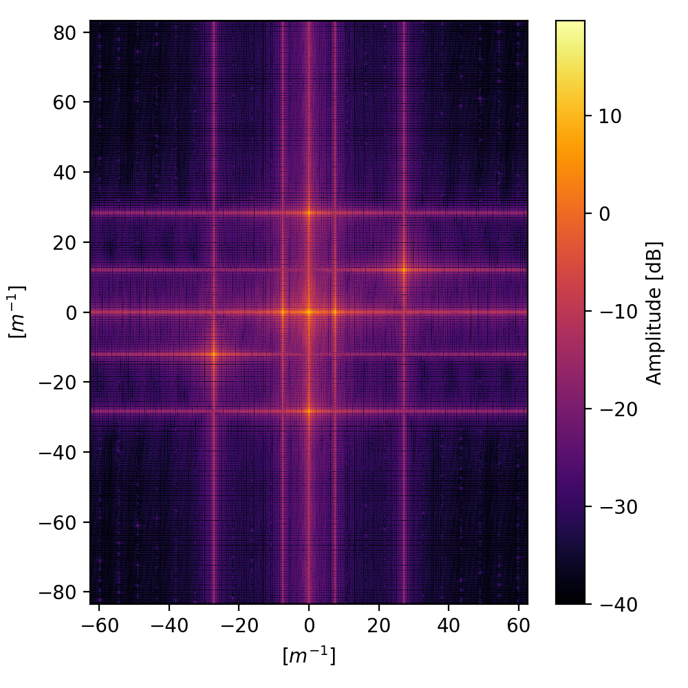
# Performing fast fourier transform
fft_matrix_2d = np.fft.fft2(matrix_2d, s=(2**11, 2**11))
# f = [-N/2, ..., -1, 0, 1, ..., N/2-1] / (Ts*N) if N is even
# f = [-(N-1)/2, ..., -1, 0, 1, ..., (N-1)/2] / (Ts*N) if N is odd
f_x = np.fft.fftshift(np.fft.fftfreq(fft_matrix_2d.shape[0], Ts_x))
f_y = np.fft.fftshift(np.fft.fftfreq(fft_matrix_2d.shape[1], Ts_y))
abs_fft_unshifted = np.abs(fft_matrix_2d)
angle_fft_unshifted = np.angle(fft_matrix_2d)
abs_fft = np.fft.fftshift(abs_fft_unshifted)
angle_fft = np.fft.fftshift(angle_fft_unshifted)
# Fourier Series Coefficients Normalization
abs_fft_norm = abs_fft / (N_x * N_y)
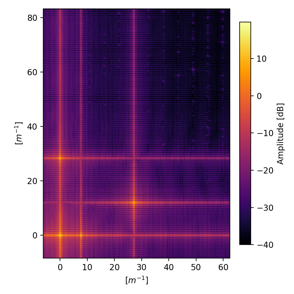
# Plotting the fft of the 2d data (in this case the image)
fig = plt.figure(figsize=(5, 5), tight_layout=True)
ax1 = fig.add_subplot(111)
fft_plot = ax1.pcolormesh(f_x, f_y, 10.0*np.log10(abs_fft_norm), cmap="inferno", vmin=-40)
# fft_plot = ax1.pcolormesh(f_x, f_y, abs_fft, vmax=5)
ax1.set_xlabel(r'$[m^{-1}]$')
ax1.set_ylabel(r'$[m^{-1}]$')
bar = plt.colorbar(fft_plot)
bar.set_label("Amplitude [dB]")
ax1.set_aspect(1)
fig.savefig("fft_2d.png", dpi=200)
plt.close(fig)
# Plotting the useful part of fft (real data)
fig = plt.figure(figsize=(5, 5), tight_layout=True)
ax1 = fig.add_subplot(111)
ind_fx0 = np.argmin(np.abs(f_x))
ind_fy0 = np.argmin(np.abs(f_y))
off_ind_fx0 = int(0.05*len(f_x))
off_ind_fy0 = int(0.05*len(f_y))
fft_plot = ax1.pcolormesh( f_x[ind_fx0-off_ind_fx0:],
                            f_y[ind_fy0-off_ind_fy0:],
                            10.0*np.log10(abs_fft_norm[ind_fx0-off_ind_fx0:, ind_fy0-off_ind_fy0:]),
                            cmap="inferno", vmin=-40)
ax1.set_xlabel(r'$[m^{-1}]$')
ax1.set_ylabel(r'$[m^{-1}]$')
ax1.set_aspect('equal')
bar = plt.colorbar(fft_plot, fraction=0.046, pad=0.04)
bar.set_label("Amplitude [dB]")
fig.savefig("fft_2d_zoomed.png", dpi=200)
plt.close(fig)
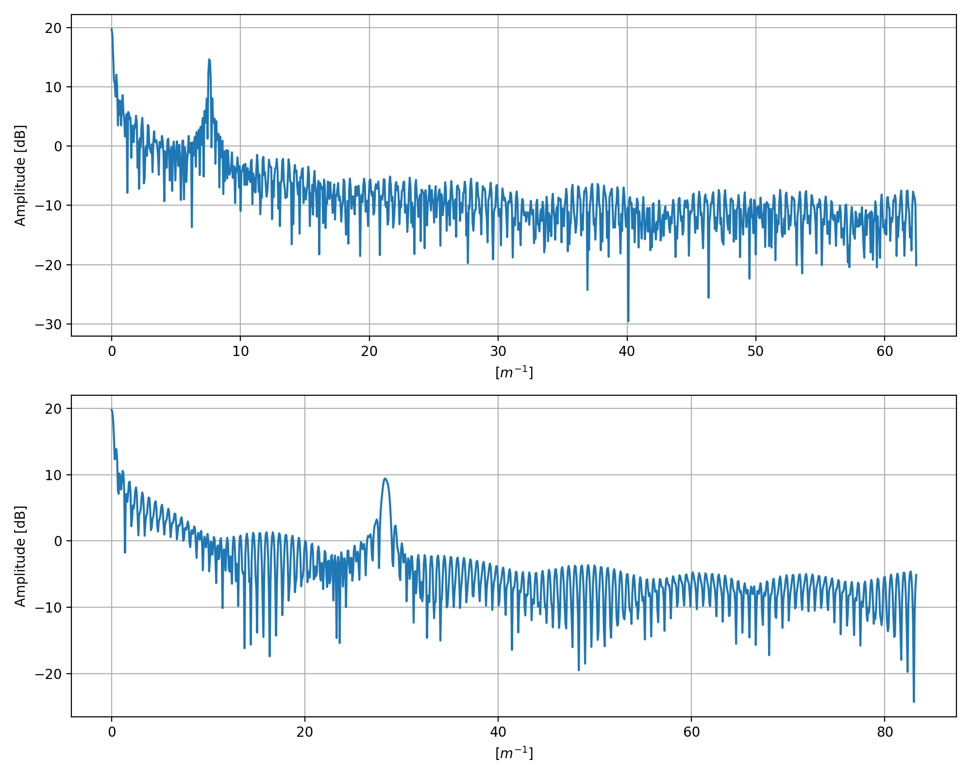
# Studing the amplitudes
Z = 10.0*np.log10(abs_fft_norm[ind_fx0:, ind_fy0:])
X = f_x[ind_fx0:]
Y = f_y[ind_fy0:]

fig = plt.figure(figsize=(10, 8), tight_layout=True)
ax1 = fig.add_subplot(211)
ax1.plot(X, Z[0, :])
ax1.set_xlabel(r'$[m^{-1}]$')
ax1.set_ylabel("Amplitude [dB]")
ax1.grid()
ax2 = fig.add_subplot(212)
ax2.set_title("FFT h")
ax2.plot(Y, Z[:, 0])
ax2.set_xlabel(r'$[m^{-1}]$')
ax2.set_ylabel("Amplitude [dB]")
ax2.grid()
fig.savefig("zoom_on.png", dpi=200)
plt.close(fig)
FFT 2D explained:
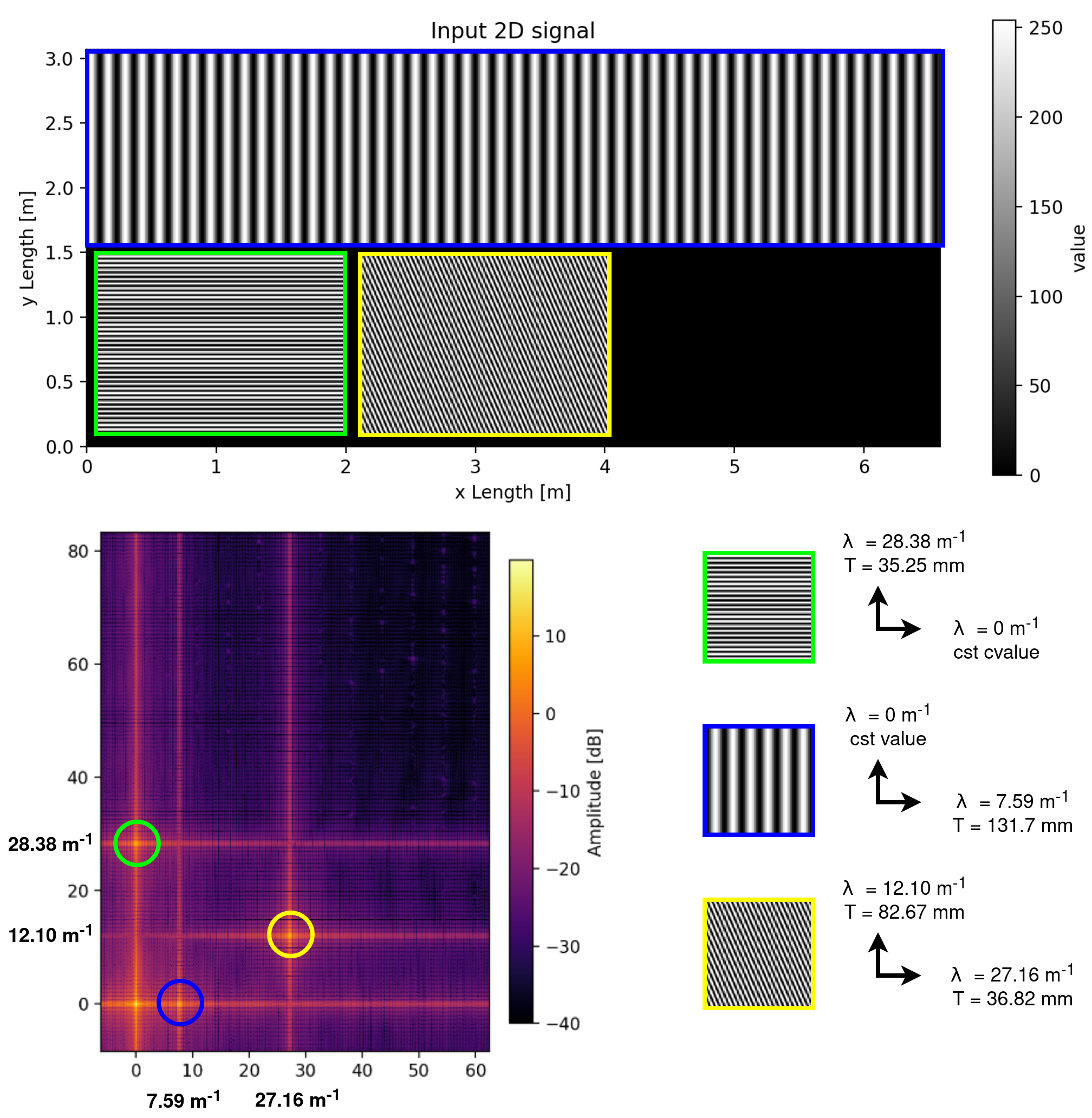
Generation of the input image above:
# Generation of the test image
import numpy as np
from PIL import Image as PImage

resolution = (512, 823) # (Height, Length)

img_data = np.zeros(resolution, dtype=np.uint8)

tmp = (np.sin(np.arange(resolution[1]) * (2 * np.pi / resolution[1]) * 50) + 1) * (255 / 2)
img_data[5:250, :] = tmp.astype(np.uint8)

tmp = (np.sin(np.arange(235) * (2 * np.pi / 235) * 40) + 1) * (255 / 2)
img_data[265:500, 10:250] = np.repeat(tmp[:, np.newaxis], 240, axis=1).astype(np.uint8)

for k in range(0, 240):
    tmp = (np.sin(np.arange(235) * (2 * np.pi / 235) * 17 - k * (np.pi / 2.3)) + 1) * (255 / 2)
    img_data[265:500, 265 + k] = tmp

img = PImage.fromarray(img_data)
img.save("example.png")
FFT Normalization Explained
TO DO:
FFT computing Fourier Series Coefficients: / N
FFT approximating a continuous Fourier Transform integral: 1/Fs
FFT preserving signal energy (Pareseval’s theorem): 1/sqrt(N)