Multilayer Perceptron

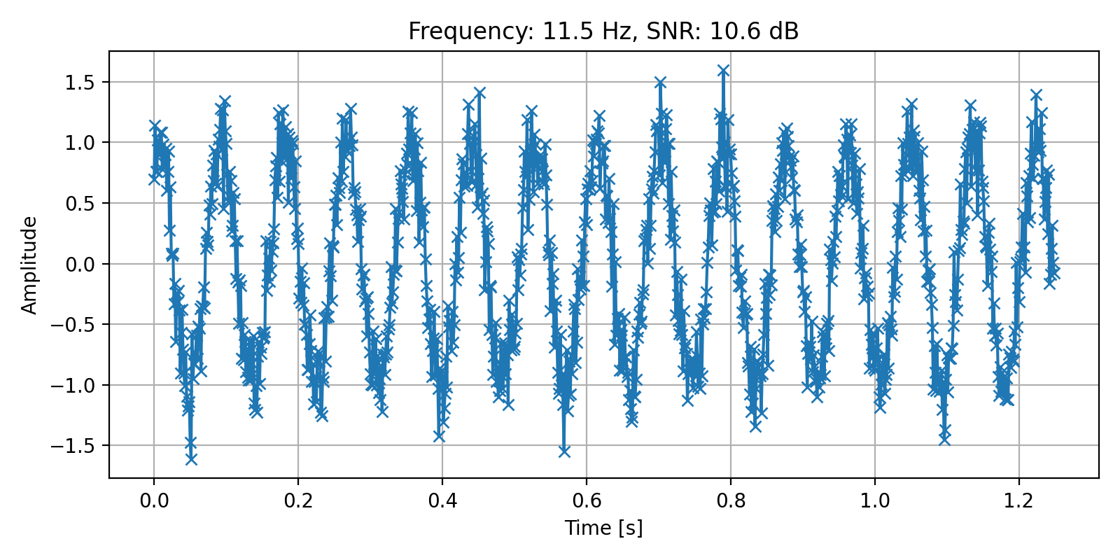
Below is a basic example of an multilayer perceptron neural network implemented with PyTorch and Tensorflow 2. As an example, we build a dataset of 1D sinus signals, the goal of the network is to recover the frequency of that signal.

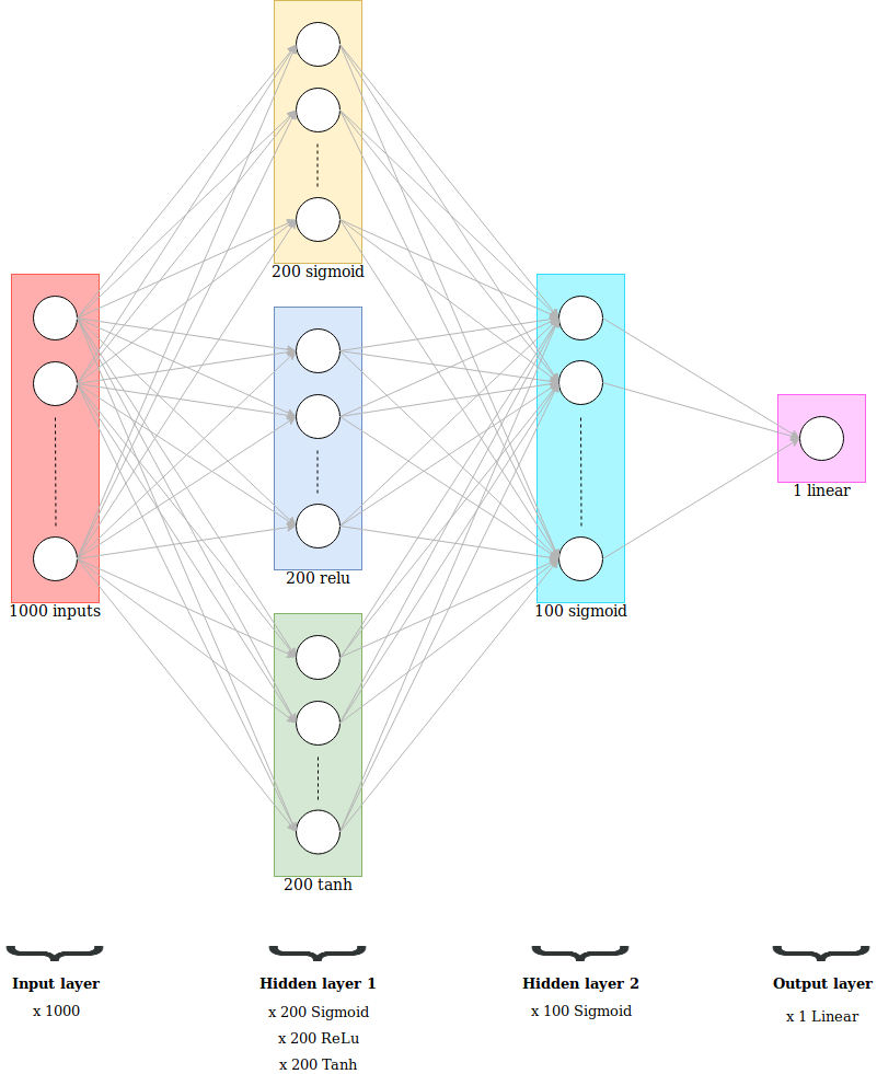
Below is the architecture of the network:

Below is the code to create the dataset:

import numpy as np
import matplotlib.pyplot as plt
from sklearn.model_selection import train_test_split
from sklearn.preprocessing import StandardScaler


# Creating the dataset
###############################################################################
# x = random sinusoidal signal in between 1 and 100hz
# y = frequency of the signals
NbPoints = 1000
fmin_hz = 1
fmax_hz = 100
fs_hz = 800.0

f_list = []
snr_list = []
x_list = []
for k in range(0, 20000):
    # Random frequency and phase
    frequency = np.random.rand(1) * (fmax_hz - fmin_hz) + fmin_hz
    phase = np.random.rand(1) * np.pi * 2
    # Signal
    x_temp = np.sin(2 * np.pi * frequency * np.arange(0, NbPoints) * (1. / fs_hz) + phase)
    # Adding noise
    signal_power_dB = 10.0 * np.log10(np.sum(np.power(x_temp, 2)) / len(x_temp))
    snr_db = np.random.randn(1) * 3 + 15
    noise_power = np.power(10.0, (signal_power_dB - snr_db) / 10.0)
    noise = np.random.normal(loc=0, scale=np.sqrt(noise_power), size=NbPoints)
    x_temp += noise
    # Adding the new data to the array
    f_list.append(frequency)
    snr_list.append(snr_db)
    x_list.append(x_temp)

X = np.array(x_list)
y = np.array(f_list).reshape((len(f_list), 1))

# Plotting a sample of one input
fig = plt.figure(figsize=(8, 4), tight_layout=True)
ax1 = fig.add_subplot(111)
ax1.plot(np.arange(1000) * 1/fs_hz, X[0], '-x')
ax1.grid()
ax1.set_xlabel("Time [s]")
ax1.set_ylabel("Amplitude")
ax1.set_title("Frequency: %.1f Hz, SNR: %.1f dB" % (f_list[0], snr_list[0]))
fig.savefig("input_sample.png", dpi=200)

# Pre-Processing
###############################################################################
# Splitting the dataset into the training set and test set
X_train, X_test, y_train, y_test = train_test_split(X, y, test_size=0.2)
# Features scaling
sc_y = StandardScaler()
y_train = sc_y.fit_transform(y_train.reshape(-1, 1))
y_test = sc_y.transform(y_test.reshape(-1, 1))


# Learning Parameters
###############################################################################
learning_rate = 0.01
nb_epochs = 50
batch_size = 500 # Better practice to take a multiple a number so that batch_size % X_train.shape[0] = 0
p_dropout = 0.25 # probability to be zeroed
# Number of iterations = nb_epochs * X_train.shape[0] / batch_size

Example of an input:

Using PyTorch

Version of Pytorch used: 1.12.1

import numpy as np
import matplotlib.pyplot as plt
import torch
import torch.nn as nn
from torch.utils.data import Dataset, DataLoader


# Creating the model
###############################################################################
device = torch.device('cuda' if torch.cuda.is_available() else 'cpu')


class MLP(nn.Module):
    def __init__(self, p_dropout:float):
        super(MLP, self).__init__()
        self.l1_sigmoid = nn.Linear(1000, 200)
        self.l1_relu = nn.Linear(1000, 200)
        self.l1_tanh = nn.Linear(1000, 200)
        self.l2_sigmoid = nn.Linear(600, 100)
        self.out_linear = nn.Linear(100, 1)
        self.dropout = nn.Dropout(p_dropout)
        self.sigmoid = nn.Sigmoid()
        self.relu = nn.ReLU()
        self.tanh = nn.Tanh()
        ### If you want to initialize weights (not recommended as pytorch is already doing it for you)
        # def init_weights(m):
        #     if isinstance(m, nn.Linear):
        #         torch.nn.init.normal_(m.weight)
        #         torch.nn.init.normal_(m.bias)
        # self.apply(init_weights)
        ### By default: model parameters are single precision float (float32)
        # Input data must match the type of the model
        # you can convert the model to double by adding self.double()

    def forward(self, x):
        l1_1 = self.dropout(self.sigmoid(self.l1_sigmoid(x)))
        l1_2 = self.dropout(self.relu(self.l1_relu(x)))
        l1_3 = self.dropout(self.tanh(self.l1_tanh(x)))
        l1 = torch.cat((l1_1, l1_2, l1_3), 1)
        l2 = self.dropout(self.l2_sigmoid(l1))
        out = self.out_linear(l2)
        return out


# Prepare the DataLoader
###############################################################################
class SinusDataset(Dataset):
    def __init__(self, x, y):
        self.x = x
        self.y = y

    def __len__(self):
        return self.x.shape[0]

    def __getitem__(self, ind):
        return self.x[ind], self.y[ind]

train_set = SinusDataset(X_train, y_train)
test_set = SinusDataset(X_test, y_test)
train_loader = DataLoader(train_set, batch_size=batch_size, shuffle=True)
test_loader = DataLoader(test_set, batch_size=batch_size, shuffle=False)


# Train the model
###############################################################################
model = MLP(p_dropout).to(device)
optimizer = torch.optim.Adam(model.parameters(), lr=learning_rate)
loss = nn.MSELoss() # nn.CrossEntropyLoss()

model.train() # Set the model in training mode
for num_epoch in range(nb_epochs):
    losses = []
    for batch_num, (x, y) in enumerate(train_loader):
        optimizer.zero_grad()
        x = x.to(device).float()
        y = y.to(device).float()
        output = model(x)
        batch_loss = loss(output, y)
        batch_loss.backward()
        losses.append(batch_loss.item())
        optimizer.step()
        if batch_num % 10 == 0:
            print(f"\tEpoch {num_epoch: 3d} | Batch {batch_num: 4d} | Loss {batch_loss.item():9.5f}")
    model.eval() # Set the model in evaluation mode (ignoring dropouts)
    losses_test = []
    for xt, yt in test_loader:
        xt = xt.to(device).float()
        yt = yt.to(device).float()
        output = model(xt)
        batch_loss = loss(output, yt)
        losses_test.append(batch_loss.item())
    print(f"Epoch {num_epoch: 3d} | Loss Training {sum(losses)/len(losses):9.5f} | Loss Testing {sum(losses_test)/len(losses_test):9.5f}")
    model.train()

print("Optimization Finished!")


# Printing and plotting the results
###############################################################################
model.eval()
y_pred = []
for xt, _ in test_loader:
    xt = xt.to(device).float()
    output = model(xt)
    output = output.cpu().detach().numpy().flatten().tolist()
    y_pred += output
# Predicting the test set results
f_target = sc_y.inverse_transform(np.array(y_test).reshape(-1, 1)).reshape(len(y_test))
f_prediction = sc_y.inverse_transform(np.array(y_pred).reshape(-1, 1)).reshape(len(y_pred))
# Mean Error
mean_error = np.mean(np.abs(f_target - f_prediction))
# Std Error
std_error = np.std(np.abs(f_target - f_prediction))
print("Error => Mean: ", mean_error, " Hz; Std: ", std_error, " Hz")


# Plotting the results
fig = plt.figure(figsize=(6, 4), tight_layout=True)
ax1 = fig.add_subplot(111)
ax1.plot(f_target, f_prediction, 'x', label="Estimations")
ax1.plot([fmin_hz, fmax_hz], [fmin_hz, fmax_hz], color='r', linewidth=2.0, label="Ideal results")
ax1.grid()
ax1.legend()
ax1.set_xlabel("Frequency to retrieve [Hz]")
ax1.set_ylabel("Frequency estimated [Hz]")
fig.savefig("NN_Predictions_pt.png", dpi=200)

Output:

        Epoch  48 | Batch    0 | Loss   0.02454
        Epoch  48 | Batch   10 | Loss   0.01721
        Epoch  48 | Batch   20 | Loss   0.01702
        Epoch  48 | Batch   30 | Loss   0.01840
Epoch  48 | Loss Training   0.01855 | Loss Testing   0.00471
        Epoch  49 | Batch    0 | Loss   0.01963
        Epoch  49 | Batch   10 | Loss   0.01530
        Epoch  49 | Batch   20 | Loss   0.01620
        Epoch  49 | Batch   30 | Loss   0.01977
Epoch  49 | Loss Training   0.01787 | Loss Testing   0.00491
Optimization Finished!
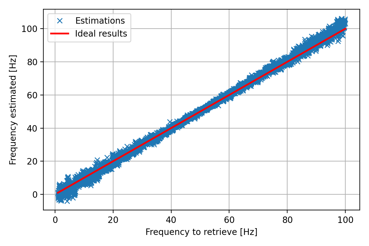
Error => Mean:  1.4843882384548015  Hz; Std:  1.3487631633755306  Hz

Results on the test dataset:

Using Tensorflow

Version of Tensorflow used: 2.9.0

import numpy as np
from sklearn.utils import shuffle
import tensorflow as tf
import matplotlib.pyplot as plt


# Creating the model
###############################################################################
class MLP():
    def __init__(self, p_dropout:float):
        self.p_dropout = p_dropout
        self.num_input = 1000
        self.n_hidden_1_1 = 200
        self.n_hidden_1_2 = 200
        self.n_hidden_1_3 = 200
        self.n_hidden_2 = 100
        self.num_output = 1

        self.params = []
        # Store layers weight & bias
        self.w_h1_1 = tf.Variable(tf.random.normal([self.num_input, self.n_hidden_1_1]), trainable=True , dtype=tf.float32)
        self.b_b1_1 = tf.Variable(tf.random.normal([self.n_hidden_1_1]), trainable=True , dtype=tf.float32)

        self.w_h1_2 = tf.Variable(tf.random.normal([self.num_input, self.n_hidden_1_2]), trainable=True , dtype=tf.float32)
        self.b_b1_2 = tf.Variable(tf.random.normal([self.n_hidden_1_2]), trainable=True , dtype=tf.float32)

        self.w_h1_3 = tf.Variable(tf.random.normal([self.num_input, self.n_hidden_1_3]), trainable=True , dtype=tf.float32)
        self.b_b1_3 = tf.Variable(tf.random.normal([self.n_hidden_1_3]), trainable=True , dtype=tf.float32)

        self.w_h2 = tf.Variable(tf.random.normal([self.n_hidden_1_1 + self.n_hidden_1_2 + self.n_hidden_1_3, self.n_hidden_2]), trainable=True , dtype=tf.float32)
        self.b_b2 = tf.Variable(tf.random.normal([self.n_hidden_2]), trainable=True , dtype=tf.float32)

        self.w_out = tf.Variable(tf.random.normal([self.n_hidden_2, self.num_output]), trainable=True , dtype=tf.float32)
        self.b_out = tf.Variable(tf.random.normal([self.num_output]), trainable=True , dtype=tf.float32)

        self.params = [ self.w_h1_1, self.b_b1_1,
                        self.w_h1_2, self.b_b1_2,
                        self.w_h1_3, self.b_b1_3,
                        self.w_h2, self.b_b2,
                        self.w_out, self.b_out]

    def parameters(self):
        return self.params

    def forward(self, x):
        # Hidden fully connected layer
        layer_1_1 = tf.nn.relu(tf.add(tf.matmul(x, self.w_h1_1), self.b_b1_1))
        do1_1 = tf.nn.dropout(layer_1_1, rate=self.p_dropout)
        layer_1_2 = tf.nn.tanh(tf.add(tf.matmul(x, self.w_h1_2), self.b_b1_2))
        do1_2 = tf.nn.dropout(layer_1_2, rate=self.p_dropout)
        layer_1_3 = tf.nn.sigmoid(tf.add(tf.matmul(x, self.w_h1_3), self.b_b1_3))
        do1_3 = tf.nn.dropout(layer_1_3, rate=self.p_dropout)
        do1 = tf.concat([do1_1, do1_2, do1_3], axis=1)
        layer_2 = tf.nn.sigmoid(tf.add(tf.matmul(do1, self.w_h2), self.b_b2))
        do2 = tf.nn.dropout(layer_2, rate=self.p_dropout)
        # Output fully connected layer with a neuron
        out_layer = tf.matmul(do2, self.w_out) + self.b_out
        return out_layer


# Train the model
###############################################################################
model = MLP(p_dropout)
optimizer = tf.optimizers.Adam(learning_rate=learning_rate)
def loss(y_pred, y_true):
    return tf.reduce_mean(tf.pow(y_pred - y_true, 2))


for num_epoch in range(nb_epochs):
    X_train, y_train = shuffle(X_train, y_train)
    for batch_num in range(0, int(np.ceil(X_train.shape[0] / batch_size))):
        batch_x = X_train[batch_num * batch_size: (batch_num + 1) * batch_size, :]
        batch_y = y_train[batch_num * batch_size: (batch_num + 1) * batch_size, :]
        with tf.GradientTape() as tape:
            batch_loss = loss(model.forward(batch_x.astype(np.float32)), batch_y.astype(np.float32))
        grads = tape.gradient(batch_loss, model.parameters())
        optimizer.apply_gradients(zip(grads, model.parameters()))
        if batch_num % 10 == 0:
            print(f"\tEpoch {num_epoch: 3d} | Batch {batch_num: 4d} | Loss {tf.reduce_mean(batch_loss):9.5f}")
    train_loss = loss(model.forward(X_train.astype(np.float32)), y_train.astype(np.float32))
    test_loss = loss(model.forward(X_test.astype(np.float32)), y_test.astype(np.float32))
    print(f"Epoch {num_epoch: 3d} | Loss Training {tf.reduce_mean(train_loss):9.5f} | Loss Testing {tf.reduce_mean(test_loss):9.5f}")

print("Optimization Finished!")


# Printing and plotting the results
###############################################################################
y_pred = model.forward(X_test.astype(np.float32))
y_pred = y_pred.numpy().flatten()
# Predicting the test set results
f_target = sc_y.inverse_transform(np.array(y_test).reshape(-1, 1)).reshape(len(y_test))
f_prediction = sc_y.inverse_transform(np.array(y_pred).reshape(-1, 1)).reshape(len(y_pred))
# Mean Error
mean_error = np.mean(np.abs(f_target - f_prediction))
# Std Error
std_error = np.std(np.abs(f_target - f_prediction))
print("Error => Mean: ", mean_error, " Hz; Std: ", std_error, " Hz")


# Plotting the results
fig = plt.figure(figsize=(6, 4), tight_layout=True)
ax1 = fig.add_subplot(111)
ax1.plot(f_target, f_prediction, 'x', label="Estimations")
ax1.plot([fmin_hz, fmax_hz], [fmin_hz, fmax_hz], color='r', linewidth=2.0, label="Ideal results")
ax1.grid()
ax1.legend()
ax1.set_xlabel("Frequency to retrieve [Hz]")
ax1.set_ylabel("Frequency estimated [Hz]")
fig.savefig("NN_Predictions_tf.png", dpi=200)

Output:

        Epoch  48 | Batch    0 | Loss   0.14032
        Epoch  48 | Batch   10 | Loss   0.15023
        Epoch  48 | Batch   20 | Loss   0.12707
        Epoch  48 | Batch   30 | Loss   0.14503
Epoch  48 | Loss Training   0.13636 | Loss Testing   0.13928
        Epoch  49 | Batch    0 | Loss   0.13721
        Epoch  49 | Batch   10 | Loss   0.12454
        Epoch  49 | Batch   20 | Loss   0.12983
        Epoch  49 | Batch   30 | Loss   0.13447
Epoch  49 | Loss Training   0.13164 | Loss Testing   0.13297
Optimization Finished!
Error => Mean:  8.441536400183606  Hz; Std:  6.459222732015336  Hz

Results on the test dataset:

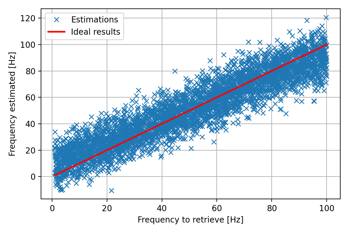
Note

Tensorflow gets worse estimations because we set manually the initialization of the weights with a normal distribution whereas PyTorch automatically initialize the weights with the “best” method.

---

Sources:

• PyTorch Documentation: https://pytorch.org/docs/stable/index.html

• Pytorch: Where to declare layers ? init ? forward ? https://stackoverflow.com/questions/50376463/pytorch-whats-the-difference-between-define-layer-in-init-and-directly-us

• PyTorch: Multilayer Perceptron By Xinhe Zhang https://medium.com/deep-learning-study-notes/multi-layer-perceptron-mlp-in-pytorch-21ea46d50e62

• PyTorch: Dataset and DataLoader: https://pytorch.org/tutorials/beginner/basics/data_tutorial.html

• Tensorflow Documentation: https://www.tensorflow.org/api_docs/python/tf/all_symbols

• Tensorflow: Image Classification With TensorFlow 2.0 By Shubham Panchal https://becominghuman.ai/image-classification-with-tensorflow-2-0-without-keras-e6534adddab2

• Tensorflow: CNN with Cifar10 https://colab.research.google.com/github/LAVI-USP/Machine-Learning/blob/master/Deep%20Learning/Classifiers/CNN_cifar10_TF2.ipynb

• Tensorflow: How to write a Neural Network in Tensorflow from scratch By Hitesh Vaidya https://medium.com/analytics-vidhya/how-to-write-a-neural-network-in-tensorflow-from-scratch-without-using-keras-e056bb143d78